Concept Of Sampling, Quantization And Resolutions
Conversion of analog signal to digital signal:
The output of most of the image sensors is an analog signal, and we can not apply digital processing on it because we can not store it. We can not store it because it requires infinite memory to store a signal that can have infinite values. So we have to convert an analog signal into a digital signal. To create an image which is digital, we need to covert continuous data into digital form. There are two steps in which it is done.
- Sampling
- Quantization
We will discuss sampling now, and quantization will be discussed later on but for now on we will discuss just a little about the difference between these two and the need of these two steps.
Basic idea:
The basic idea behind converting an analog signal to its digital signal is

to convert both of its axis x,yx,y into a digital format. Since an image is continuous not just in its co-ordinates xaxisxaxis, but also in its amplitude yaxisyaxis, so the part that deals with the digitizing of co-ordinates is known as sampling. And the part that deals with digitizing the amplitude is known as quantization.
Sampling.
The term sampling refers to take samples. We digitize x axis in sampling. It is done on independent variable. In case of, equation y = sinx, it is done on x variable. It is further divided into two parts , up sampling and down sampling
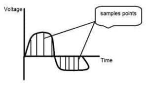
If you will look at the above figure, you will see that there are some random variations in the signal. These variations are due to noise. In sampling we reduce this noise by taking samples. It is obvious that more samples we take, the quality of the image would be more better, the noise would be more removed and same happens vice versa.
However, if you take sampling on the x axis, the signal is not converted to digital format, unless you take sampling of the y-axis too which is known as quantization. The more samples eventually means you are collecting more data, and in case of image, it means more pixels.
Relationship with pixels
Since a pixel is a smallest element in an image. The total number of pixels in an image can be calculated as
Pixels = total no of rows * total no of columns.
Lets say we have total of 25 pixels, that means we have a square image of 5 X 5. Then as we have discussed above in sampling, that more samples eventually result in more pixels. So it means that of our continuous signal, we have taken 25 samples on x axis. That refers to 25 pixels of this image. This leads to another conclusion that since pixel is also the smallest division of a CCD array. So it means it has a relationship with CCD array too, which can be explained as this.
Relationship with CCD array
The number of sensors on a CCD array is directly equal to the number of pixels. And since we have concluded that the number of pixels is directly equal to the number of samples, that means that number sample is directly equal to the number of sensors on CCD array.
Oversampling.
In the beginning we have define that sampling is further categorize into two types. Which is up sampling and down sampling. Up sampling is also called as over sampling. The oversampling has a very deep application in image processing which is known as Zooming.
Zooming
We will formally introduce zooming in the upcoming tutorial, but for now on, we will just briefly explain zooming. Zooming refers to increase the quantity of pixels, so that when you zoom an image, you will see more detail. The increase in the quantity of pixels is done through oversampling. The one way to zoom is, or to increase samples, is to zoom optically, through the motor movement of the lens and then capture the image. But we have to do it, once the image has been captured.
There is a difference between zooming and sampling
The concept is same, which is, to increase samples. But the key difference is that while sampling is done on the signals, zooming is done on the digital image.
Quantization
Digitizing a signal
As we have seen in the previous tutorials, that digitizing an analog signal into a digital, requires two basic steps. Sampling and quantization. Sampling is done on x axis. It is the conversion of x axis infinite values to digital values. The below figure shows sampling of a signal.
Sampling with relation to digital images
The concept of sampling is directly related to zooming. The more samples you take, the more pixels, you get. Oversampling can also be called as zooming. This has been discussed under sampling and zooming tutorial.But the story of digitizing a signal does not end at sampling too, there is another step involved which is known as Quantization.
What is quantization
Quantization is opposite to sampling. It is done on y axis. When you are quantizing an image, you are actually dividing a signal into quantapartitions. On the x axis of the signal, are the co-ordinate values, and on the y axis, we have amplitudes. So digitizing the amplitudes is known as Quantization.
Here how it is done
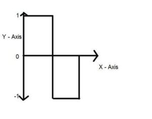
You can see in this image, that the signal has been quantified into three different levels. That means that when we sample an image, we actually gather a lot of values, and in quantization, we set levels to these values. This can be more clear in the image below.

In the figure shown in sampling, although the samples has been taken, but they were still spanning vertically to a continuous range of gray level values. In the figure shown above, these vertically ranging values have been quantized into 5 different levels or partitions. Ranging from 0 black to 4 white. This level could vary according to the type of image you want.
The relation of quantization with gray levels has been further discussed below.
Relation of Quantization with gray level resolution:
The quantized figure shown above has 5 different levels of gray. It means that the image formed from this signal, would only have 5 different colors. It would be a black and white image more or less with some colors of gray. Now if you were to make the quality of the image more better, there is one thing you can do here. Which is, to increase the levels, or gray level resolution up. If you increase this level to 256, it means you have an gray scale image. Which is far better then simple black and white image. Now 256, or 5 or what ever level you choose is called gray level. Remember the formula that we discussed in the previous tutorial of gray level resolution which is,
L= 2^k
We have discussed that gray level can be defined in two ways. Which were these two.
- Gray level = number of bits per pixel BPPBPP.
- Gray level = number of levels per pixel.
In this case we have gray level is equal to 256. If we have to calculate the number of bits, we would simply put the values in the equation. In case of 256levels, we have 256 different shades of gray and 8 bits per pixel, hence the image would be a gray scale image.
Reducing the gray level
Now we will reduce the gray levels of the image to see the effect on the image.
For example
Lets say you have an image of 8bpp, that has 256 different levels. It is a grayscale image and the image looks something like this.
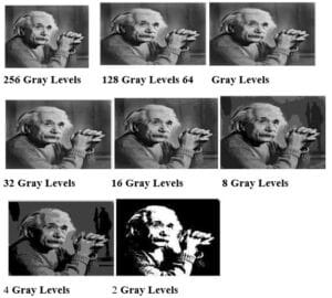
256 Gray Levels
Now we will start reducing the gray levels. We will first reduce the gray levels from 256 to 128.
128 Gray Levels
There is not much effect on an image after decrease the gray levels to its half. Lets decrease some more.
64 Gray Levels
Still not much effect, then lets reduce the levels more.
32 Gray Levels
Surprised to see, that there is still some little effect. May be its due to reason, that it is the picture of Einstein, but lets reduce the levels more.
16 Gray Levels
Boom here, we go, the image finally reveals, that it is effected by the levels.
8 Gray Levels
4 Gray Levels
Now before reducing it, further two 2 levels, you can easily see that the image has been distorted badly by reducing the gray levels. Now we will reduce it to 2 levels, which is nothing but a simple black and white level. It means the image would be simple black and white image.
2 Gray Levels
Thats the last level we can achieve, because if reduce it further, it would be simply a black image, which can not be interpreted.
Contouring
There is an interesting observation here, that as we reduce the number of gray levels, there is a special type of effect start appearing in the image, which can be seen clear in 16 gray level picture. This effect is known as Contouring.
Image Resolution
Image resolution can be defined in many ways. One type of it which is pixel resolution that has been discussed in the tutorial of pixel resolution and aspect ratio.
Spatial resolution
Spatial resolution states that the clarity of an image cannot be determined by the pixel resolution. The number of pixels in an image does not matter. Spatial resolution can be defined as the in other way we can define spatial resolution as the number of independent pixels values per inch. In short what spatial resolution refers to is that we cannot compare two different types of images to see that which one is clear or which one is not. If we have to compare the two images, to see which one is more clear or which has more spatial resolution, we have to compare two images of the same size.
For example:
You cannot compare these two images to see the clarity of the image.

Although both images are of the same person, but that is not the condition we are judging on. The picture on the left is zoomed out picture of Einstein with dimensions of 227 x 222. Whereas the picture on the right side has the dimensions of 980 X 749 and also it is a zoomed image. We cannot compare them to see that which one is more clear. Remember the factor of zoom does not matter in this condition, the only thing that matters is that these two pictures are not equal.
So in order to measure spatial resolution , the pictures below would server the purpose.

Now you can compare these two pictures. Both the pictures has same dimensions which are of 227 X 222. Now when you compare them, you will see that the picture on the left side has more spatial resolution or it is more clear then the picture on the right side. That is because the picture on the right is a blurred image.
Measuring spatial resolution
Since the spatial resolution refers to clarity, so for different devices, different measure has been made to measure it.
For example
- Dots per inch
- Lines per inch
- Pixels per inch
They are discussed in more detail in the next tutorial but just a brief introduction has been given below.
Dots per inch
Dots per inch or DPI is usually used in monitors.
Lines per inch
Lines per inch or LPI is usually used in laser printers.
Pixel per inch
Pixel per inch or PPI is measure for different devices such as tablets , Mobile phones e.t.c.
Gray level resolution
Gray level resolution refers to the predictable or deterministic change in the shades or levels of gray in an image. In short gray level resolution is equal to the number of bits per pixel. We have already discussed bits per pixel in our tutorial of bits per pixel and image storage requirements. We will define bpp here briefly.
BPP
The number of different colors in an image is depends on the depth of color or bits per pixel.
Mathematically
The mathematical relation that can be established between gray level resolution and bits per pixel can be given as.
L = 2^k
In this equation L refers to number of gray levels. It can also be defined as the shades of gray. And k refers to bpp or bits per pixel. So the 2 raise to the power of bits per pixel is equal to the gray level resolution.
For example:

The above image of Einstein is an gray scale image. Means it is an image with 8 bits per pixel or 8bpp. Now if were to calculate the gray level resolution, here how we gonna do it. It means it gray level resolution is 256. Or in other way we can say that this image has 256 different shades of gray. The more is the bits per pixel of an image, the more is its gray level resolution.
Defining gray level resolution in terms of bpp
It is not necessary that a gray level resolution should only be defined in terms of levels. We can also define it in terms of bits per pixel.
For example
If you are given an image of 4 bpp, and you are asked to calculate its gray level resolution. There are two answers to that question. The first answer is 16 levels. The second answer is 4 bits.
Finding bpp from Gray level resolution
You can also find the bits per pixels from the given gray level resolution. For this, we just have to twist the formula a little.
Equation 1.
L = 2^k
where k=8
l =2^8
L=256
This formula finds the levels. Now if we were to find the bits per pixel or in this case k, we will simply change it like this.
K = log base 2LL Equation 22
Because in the first equation the relationship between Levels LL and bits per pixel kk is exponentional. Now we have to revert it, and thus the inverse of exponentional is log. Lets take an example to find bits per pixel from gray level resolution.
For example:
If you are given an image of 256 levels. What is the bits per pixel required for it.
Putting 256 in the equation, we get.
K = log base 2 256256 K = 8.
So the answer is 8 bits per pixel.
Gray level resolution and quantization:
The quantization will be formally introduced in the next tutorial, but here we are just going to explain the relation ship between gray level resolution and quantization. Gray level resolution is found on the y axis of the signal. In the tutorial of Introduction to signals and system, we have studied that digitizing a an analog signal requires two steps. Sampling and quantization.
Sampling is done on x axis. And quantization is done in Y axis.
So that means digitizing the gray level resolution of an image is done in quantization.
0 Comments