Speech Recognition

Speech is the most basic means of adult human communication. The basic goal of speech processing is to provide an interaction between a human and a machine.

Speech processing system has mainly three tasks −

• First, speech recognition that allows the machine to catch the words, phrases and sentences we speak
• Second, natural language processing to allow the machine to understand what we speak, and
• Third, speech synthesis to allow the machine to speak.

This chapter focuses on speech recognition, the process of understanding the words that are spoken by human beings. Remember that the speech signals are captured with the help of a microphone and then it has to be understood by the system.

Building a Speech Recognizer

Speech Recognition or Automatic Speech Recognition (ASR) is the center of attention for AI projects like robotics. Without ASR, it is not possible to imagine a cognitive robot interacting with a human. However, it is not quite easy to build a speech recognizer.

Difficulties in developing a speech recognition system

Developing a high quality speech recognition system is really a difficult problem. The difficulty of speech recognition technology can be broadly characterized along a number of dimensions as discussed below −

• • Size of the vocabulary − Size of the vocabulary impacts the ease of developing an ASR. Consider the following sizes of vocabulary for a better understanding.
    • A small size vocabulary consists of 2-100 words, for example, as in a voice-menu system
    • A medium size vocabulary consists of several 100s to 1,000s of words, for example, as in a database-retrieval task
    • A large size vocabulary consists of several 10,000s of words, as in a general dictation task.

Note that, the larger the size of vocabulary, the harder it is to perform recognition.

• • Channel characteristics − Channel quality is also an important dimension. For example, human speech contains high bandwidth with full frequency range, while a telephone speech consists of low bandwidth with limited frequency range. Note that it is harder in the latter.
  • Speaking mode − Ease of developing an ASR also depends on the speaking mode, that is whether the speech is in isolated word mode, or connected word mode, or in a continuous speech mode. Note that a continuous speech is harder to recognize.
  • Speaking style − A read speech may be in a formal style, or spontaneous and conversational with casual style. The latter is harder to recognize.
  • Speaker dependency − Speech can be speaker dependent, speaker adaptive, or speaker independent. A speaker independent is the hardest to build.
  • Type of noise − Noise is another factor to consider while developing an ASR. Signal to noise ratio may be in various ranges, depending on the acoustic environment that observes less versus more background noise −
    • If the signal to noise ratio is greater than 30dB, it is considered as high range
    • If the signal to noise ratio lies between 30dB to 10db, it is considered as medium SNR
    • If the signal to noise ratio is lesser than 10dB, it is considered as low range

For example, the type of background noise such as stationary, non-human noise, background speech and crosstalk by other speakers also contributes to the difficulty of the problem.

• Microphone characteristics − The quality of microphone may be good, average, or below average. Also, the distance between mouth and micro-phone can vary. These factors also should be considered for recognition systems.

Despite these difficulties, researchers worked a lot on various aspects of speech such as understanding the speech signal, the speaker, and identifying the accents.

You will have to follow the steps given below to build a speech recognizer:

Visualizing Audio Signals:

Reading from a File and Working on it. This is the first step in building speech recognition system as it gives an understanding of how an audio signal is structured. Some common steps that can be followed to work with audio signals are as follows −

Recording

When you have to read the audio signal from a file, then record it using a microphone, at first.

Sampling

When recording with microphone, the signals are stored in a digitized form. But to work upon it, the machine needs them in the discrete numeric form. Hence, we should perform sampling at a certain frequency and convert the signal into the discrete numerical form. Choosing the high frequency for sampling implies that when humans listen to the signal, they feel it as a continuous audio signal.

Example

The following example shows a stepwise approach to analyze an audio signal, using Python, which is stored in a file. The frequency of this audio signal is 44,100 HZ.

Import the necessary packages as shown here −

import numpy as np
import matplotlib.pyplot as plt
from scipy.io import wavfile

Now, read the stored audio file. It will return two values: the sampling frequency and the audio signal. Provide the path of the audio file where it is stored, as shown here −

frequency_sampling, audio_signal = wavfile.read("/Users/admin/audio_file.wav")

Display the parameters like sampling frequency of the audio signal, data type of signal and its duration, using the commands shown −

print('\nSignal shape:', audio_signal.shape)
print('Signal Datatype:', audio_signal.dtype)
print('Signal duration:', round(audio_signal.shape[0] / 
float(frequency_sampling), 2), 'seconds')

This step involves normalizing the signal as shown below −

audio_signal = audio_signal / np.power(2, 15)

In this step, we are extracting the first 100 values from this signal to visualize. Use the following commands for this purpose −

audio_signal = audio_signal [:100]
time_axis = 1000 * np.arange(0, len(signal), 1) / float(frequency_sampling)

Now, visualize the signal using the commands given below −

plt.plot(time_axis, signal, color='blue')
plt.xlabel('Time (milliseconds)')
plt.ylabel('Amplitude')
plt.title('Input audio signal')
plt.show()

You would be able to see an output graph and data extracted for the above audio signal as shown in the image here

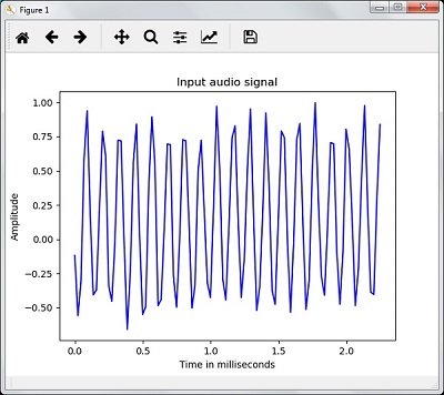
Signal shape: (132300,)
Signal Datatype: int16
Signal duration: 3.0 seconds

Characterizing the Audio Signal: Transforming to Frequency Domain

Characterizing an audio signal involves converting the time domain signal into frequency domain, and understanding its frequency components, by. This is an important step because it gives a lot of information about the signal. You can use a mathematical tool like Fourier Transform to perform this transformation.

Example

The following example shows, step-by-step, how to characterize the signal, using Python, which is stored in a file. Note that here we are using Fourier Transform mathematical tool to convert it into frequency domain.

Import the necessary packages, as shown here −

import numpy as np
import matplotlib.pyplot as plt
from scipy.io import wavfile

Now, read the stored audio file. It will return two values: the sampling frequency and the the audio signal. Provide the path of the audio file where it is stored as shown in the command here −

frequency_sampling, audio_signal = wavfile.read("/Users/admin/sample.wav")

In this step, we will display the parameters like sampling frequency of the audio signal, data type of signal and its duration, using the commands given below −

print('\nSignal shape:', audio_signal.shape)
print('Signal Datatype:', audio_signal.dtype)
print('Signal duration:', round(audio_signal.shape[0] / 
float(frequency_sampling), 2), 'seconds')

In this step, we need to normalize the signal, as shown in the following command −

audio_signal = audio_signal / np.power(2, 15)

This step involves extracting the length and half length of the signal. Use the following commands for this purpose −

length_signal = len(audio_signal)
half_length = np.ceil((length_signal + 1) / 2.0).astype(np.int)

Now, we need to apply mathematics tools for transforming into frequency domain. Here we are using the Fourier Transform.

signal_frequency = np.fft.fft(audio_signal)

Now, do the normalization of frequency domain signal and square it −

signal_frequency = abs(signal_frequency[0:half_length]) / length_signal
signal_frequency **= 2

Next, extract the length and half length of the frequency transformed signal −

len_fts = len(signal_frequency)

Note that the Fourier transformed signal must be adjusted for even as well as odd case.

if length_signal % 2:
   signal_frequency[1:len_fts] *= 2
else:
   signal_frequency[1:len_fts-1] *= 2

Now, extract the power in decibal(dB) −

signal_power = 10 * np.log10(signal_frequency)

Adjust the frequency in kHz for X-axis −

x_axis = np.arange(0, len_half, 1) * (frequency_sampling / length_signal) / 1000.0

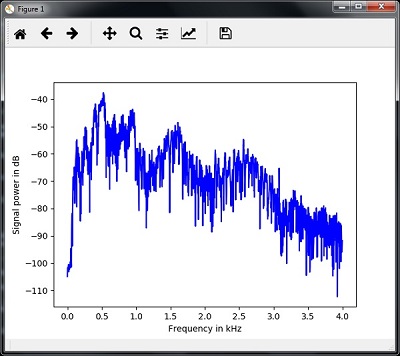
Now, visualize the characterization of signal as follows −

plt.figure()
plt.plot(x_axis, signal_power, color='black')
plt.xlabel('Frequency (kHz)')
plt.ylabel('Signal power (dB)')
plt.show()

You can observe the output graph of the above code as shown in the image below −

Generating Monotone Audio Signal

The two steps that you have seen till now are important to learn about signals. Now, this step will be useful if you want to generate the audio signal with some predefined parameters. Note that this step will save the audio signal in an output file.

Example

In the following example, we are going to generate a monotone signal, using Python, which will be stored in a file. For this, you will have to take the following steps −

Import the necessary packages as shown −

import numpy as np
import matplotlib.pyplot as plt
from scipy.io.wavfile import write

Provide the file where the output file should be saved

output_file = 'audio_signal_generated.wav'

Now, specify the parameters of your choice, as shown −

duration = 4 # in seconds
frequency_sampling = 44100 # in Hz
frequency_tone = 784
min_val = -4 * np.pi
max_val = 4 * np.pi

In this step, we can generate the audio signal, as shown −

t = np.linspace(min_val, max_val, duration * frequency_sampling)
audio_signal = np.sin(2 * np.pi * tone_freq * t)

Now, save the audio file in the output file −

write(output_file, frequency_sampling, signal_scaled)

Extract the first 100 values for our graph, as shown −

audio_signal = audio_signal[:100]
time_axis = 1000 * np.arange(0, len(signal), 1) / float(sampling_freq)

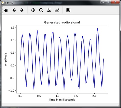
Now, visualize the generated audio signal as follows −

plt.plot(time_axis, signal, color='blue')
plt.xlabel('Time in milliseconds')
plt.ylabel('Amplitude')
plt.title('Generated audio signal')
plt.show()

You can observe the plot as shown in the figure given here −

Feature Extraction from Speech

This is the most important step in building a speech recognizer because after converting the speech signal into the frequency domain, we must convert it into the usable form of feature vector. We can use different feature extraction techniques like MFCC, PLP, PLP-RASTA etc. for this purpose.

Example

In the following example, we are going to extract the features from signal, step-by-step, using Python, by using MFCC technique.

Import the necessary packages, as shown here −

import numpy as np
import matplotlib.pyplot as plt
from scipy.io import wavfile
from python_speech_features import mfcc, logfbank

Now, read the stored audio file. It will return two values − the sampling frequency and the audio signal. Provide the path of the audio file where it is stored.

frequency_sampling, audio_signal = wavfile.read("/Users/admin/audio_file.wav")

Note that here we are taking first 15000 samples for analysis.

audio_signal = audio_signal[:15000]

Use the MFCC techniques and execute the following command to extract the MFCC features −

features_mfcc = mfcc(audio_signal, frequency_sampling)

Now, print the MFCC parameters, as shown −

print('\nMFCC:\nNumber of windows =', features_mfcc.shape[0])
print('Length of each feature =', features_mfcc.shape[1])

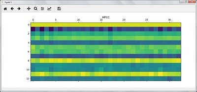
Now, plot and visualize the MFCC features using the commands given below −

features_mfcc = features_mfcc.T
plt.matshow(features_mfcc)
plt.title('MFCC')

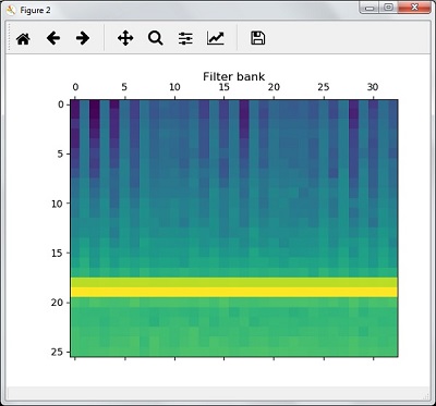
In this step, we work with the filter bank features as shown −

Extract the filter bank features −

filterbank_features = logfbank(audio_signal, frequency_sampling)

Now, print the filterbank parameters.

print('\nFilter bank:\nNumber of windows =', filterbank_features.shape[0])
print('Length of each feature =', filterbank_features.shape[1])

Now, plot and visualize the filterbank features.

filterbank_features = filterbank_features.T
plt.matshow(filterbank_features)
plt.title('Filter bank')
plt.show()

As a result of the steps above, you can observe the following outputs: Figure1 for MFCC and Figure2 for Filter Bank

Recognition of Spoken Words

Speech recognition means that when humans are speaking, a machine understands it. Here we are using Google Speech API in Python to make it happen. We need to install the following packages for this −

• Pyaudio − It can be installed by using pip install Pyaudio command.
• SpeechRecognition − This package can be installed by using pip install SpeechRecognition.
• Google-Speech-API − It can be installed by using the command pip install google-api-python-client.

Example

Observe the following example to understand about recognition of spoken words −

Import the necessary packages as shown −

import speech_recognition as sr

Create an object as shown below −

recording = sr.Recognizer()

Now, the Microphone() module will take the voice as input −

with sr.Microphone() as source: recording.adjust_for_ambient_noise(source)
   print("Please Say something:")
   audio = recording.listen(source)

Now google API would recognize the voice and gives the output.

try:
   print("You said: \n" + recording.recognize_google(audio))
except Exception as e:
   print(e)

You can see the following output −

Please Say Something:
You said:

For example, if you said tutorialspoint.com, then the system recognizes it correctly as follows −

tutorialspoint.com

[wpsbx_html_block id=1891]