Part 7: 2D Geometric Transformations: Translation, Scaling, Rotation & Matrices
Linear Algebra of Visual Manipulation
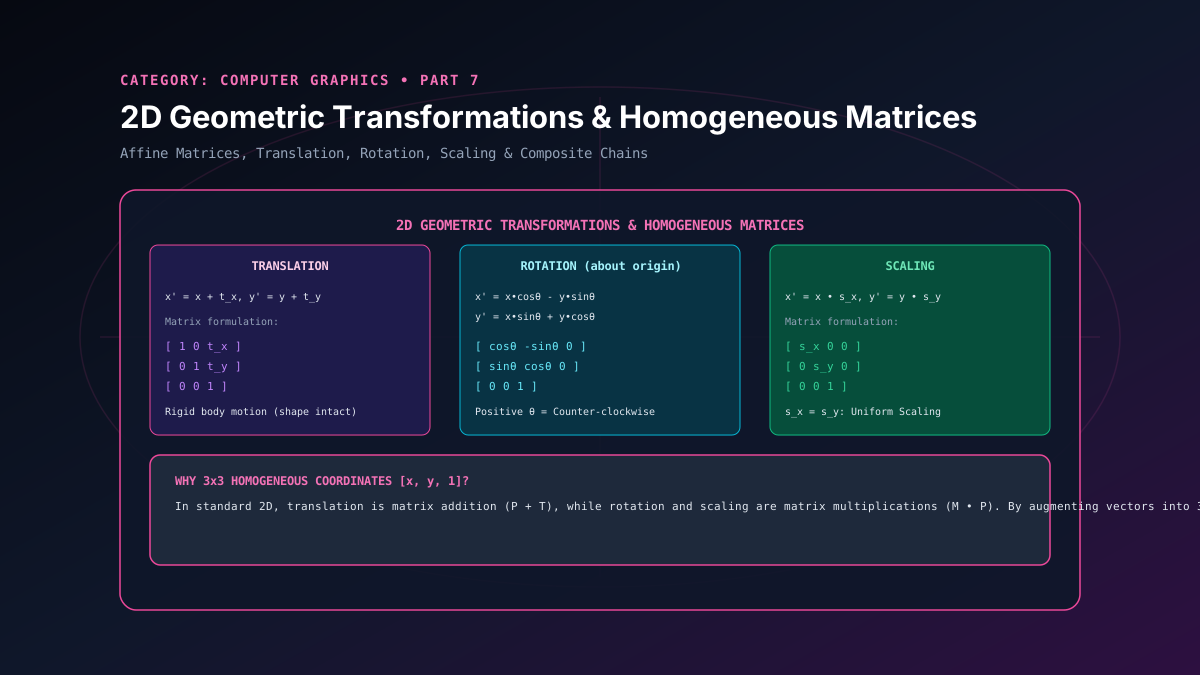
Geometric transformations are the engine of computer graphics, enabling scenes to animate, scale, rotate, and interact dynamically. While linear operations (scaling and rotation) can be represented by $2 \times 2$ matrices, translation is an affine operation that requires vector addition. To unify all affine transformations into a single mathematical formalism that can be chained via matrix multiplication, computer graphics adopts projective homogeneous coordinates. In this article, we formulate 2D transformation matrices, solve arbitrary pivot-point rotations, and demonstrate composite matrix composition.
1. Basic Affine Transformations in 2D Space
Translation
Translates a point by vector $(t_x, t_y)$:
y' = y + t_y
Scaling
Multiplies dimensions by factors $(s_x, s_y)$:
y' = y \cdot s_y
Rotation
Rotates counter-clockwise by angle $\theta$:
y' = x\sin\theta + y\cos\theta
2. Homogeneous Coordinates & $3 \times 3$ Transformation Matrices
In standard Cartesian 2D coordinates, translation cannot be expressed as a matrix multiplication with a $2 \times 2$ matrix because $x' = x + t_x$ is non-linear. By augmenting the coordinate vector with a third scale factor $w=1$, a 2D Cartesian point $(x, y)$ becomes the homogeneous vector $[x, y, 1]^T$.
In this 3-dimensional projective space, all affine transformations are unified into uniform $3 \times 3$ matrix multiplications:
Translation $T(t_x, t_y)$
[ 1   0   tx ]
[ 0   1   ty ]
[ 0   0   1  ]
Scaling $S(s_x, s_y)$
[ sx  0   0  ]
[ 0   sy  0  ]
[ 0   0   1  ]
Rotation $R( heta)$
[ cosθ -sinθ 0 ]
[ sinθ  cosθ 0 ]
[  0     0   1 ]
3. Composite Transformations: Pivot Point Rotation
A fundamental property of matrix composition is that matrix multiplication is associative but strictly non-commutative:
To rotate an object around an arbitrary pivot point $(x_r, y_r)$ rather than the coordinate origin, we execute a composite 3-step matrix sequence:
- Translate the pivot point $(x_r, y_r)$ to the origin: $T(-x_r, -y_r)$.
- Rotate by angle $\theta$ around the origin: $R(\theta)$.
- Translate the origin back to the pivot point: $T(x_r, y_r)$.
Multiplying these three matrices produces a single consolidated $3 \times 3$ transformation matrix. Any polygon containing $10,000$ vertices can now be transformed by multiplying each vertex by $M_{composite}$ once, eliminating redundant intermediate calculations.
Related reading

How to Give Google Antigravity Direct SSH Access to Remote Servers (Proxmox & Linux)
Connect Google Antigravity directly to Proxmox and Linux servers using the Model Context Protocol (MCP), dedicated Ed25519 keys, and automated updates.
By Super Admin
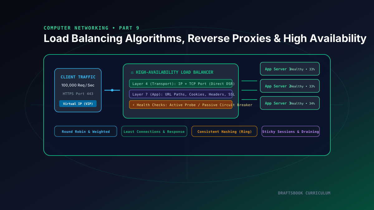
Part 9: Load Balancing: Layer 4 vs Layer 7, Algorithms, Reverse Proxies & High Availability
Master high-availability load balancing, comparing Layer 4 transport vs Layer 7 application routing, consistent hashing rings, and health checks.
By Super Admin
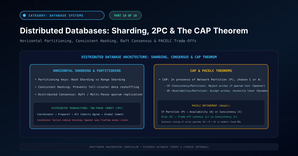
Part 10: Distributed Databases: Partitioning, Sharding, 2PC & CAP Theorem
Master distributed database architecture: horizontal sharding, consistent hashing, two-phase commit (2PC), CAP theorem trade-offs, and NewSQL engines.
By Super Admin
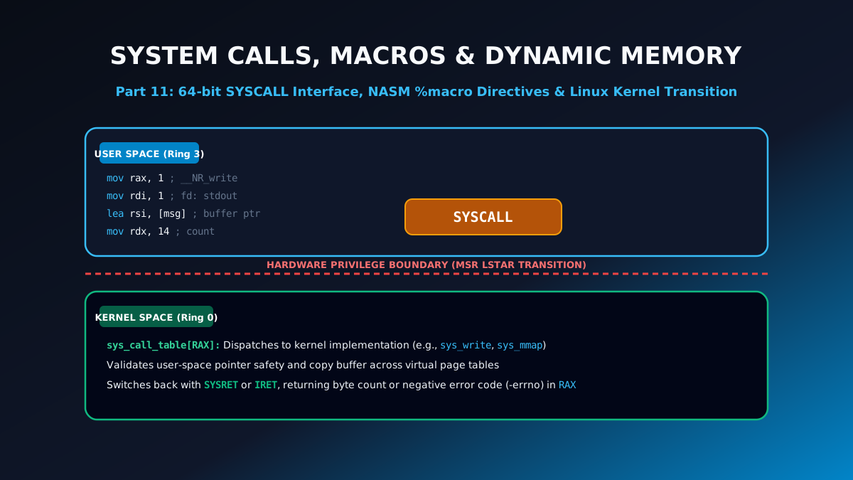
Part 11: Linux 64-Bit System Calls, NASM Macros & Dynamic Memory Allocation
Learn low-level systems programming: Linux 64-bit SYSCALL table, multi-argument NASM %macro directives, file I/O operations, and sys_mmap memory allocation.
By Super Admin