Artificial Neural Networks (ANN)

Artificial Neural network (ANN) is an efficient computing system whose central theme is borrowed from the analogy of biological neural networks. ANNs are also named as Artificial Neural Systems, Parallel Distributed Processing Systems, and Connectionist Systems. ANN acquires large collection of units that are interconnected in some pattern to allow communications between them. These units, also referred to as nodes or neurons, are simple processors which operate in parallel.

Every neuron is connected with other neuron through a connection link. Each connection link is associated with a weight having the information about the input signal. This is the most useful information for neurons to solve a particular problem because the weight usually excites or inhibits the signal that is being communicated. Each neuron is having its internal state which is called activation signal. Output signals, which are produced after combining input signals and activation rule, may be sent to other units.

[wpsbx_html_block id=1891]

If you want to study neural networks in detail then you can follow the link:

Installing Useful Packages

For creating neural networks in Python, we can use a powerful package for neural networks called NeuroLab. It is a library of basic neural networks algorithms with flexible network configurations and learning algorithms for Python. You can install this package with the help of the following command on command prompt −

pip install NeuroLab

If you are using the Anaconda environment, then use the following command to install NeuroLab −

conda install -c labfabulous neurolab

Building Neural Networks

In this section, let us build some neural networks in Python by using the NeuroLab package.

Perceptron based Classifier

Perceptrons are the building blocks of ANN. If you want to know more about Perceptron, you can follow the link − artificial_neural_network

Following is a stepwise execution of the Python code for building a simple neural network perceptron based classifier −

Import the necessary packages as shown −

import matplotlib.pyplot as plt
import neurolab as nl

Enter the input values. Note that it is an example of supervised learning, hence you will have to provide target values too.

input = [[0, 0], [0, 1], [1, 0], [1, 1]]
target = [[0], [0], [0], [1]]

Create the network with 2 inputs and 1 neuron −

net = nl.net.newp([[0, 1],[0, 1]], 1)

Now, train the network. Here, we are using Delta rule for training.

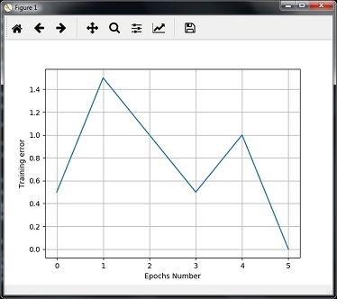
error_progress = net.train(input, target, epochs=100, show=10, lr=0.1)

Now, visualize the output and plot the graph −

plt.figure()
plt.plot(error_progress)
plt.xlabel('Number of epochs')
plt.ylabel('Training error')
plt.grid()
plt.show()

You can see the following graph showing the training progress using the error metric −

Single – Layer Neural Networks

In this example, we are creating a single layer neural network that consists of independent neurons acting on input data to produce the output. Note that we are using the text file named neural_simple.txt as our input.

Import the useful packages as shown −

import numpy as np
import matplotlib.pyplot as plt
import neurolab as nl

Load the dataset as follows −

input_data = np.loadtxt(“/Users/admin/neural_simple.txt')

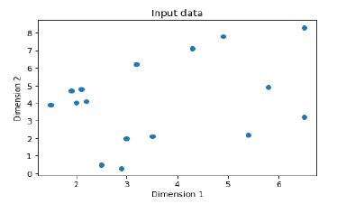
The following is the data we are going to use. Note that in this data, first two columns are the features and last two columns are the labels.

array([[2. , 4. , 0. , 0. ],
      [1.5, 3.9, 0. , 0. ],
      [2.2, 4.1, 0. , 0. ],
      [1.9, 4.7, 0. , 0. ],
      [5.4, 2.2, 0. , 1. ],
      [4.3, 7.1, 0. , 1. ],
      [5.8, 4.9, 0. , 1. ],
      [6.5, 3.2, 0. , 1. ],
      [3. , 2. , 1. , 0. ],
      [2.5, 0.5, 1. , 0. ],
      [3.5, 2.1, 1. , 0. ],
      [2.9, 0.3, 1. , 0. ],
      [6.5, 8.3, 1. , 1. ],
      [3.2, 6.2, 1. , 1. ],
      [4.9, 7.8, 1. , 1. ],
      [2.1, 4.8, 1. , 1. ]])

Now, separate these four columns into 2 data columns and 2 labels −

data = input_data[:, 0:2]
labels = input_data[:, 2:]

Plot the input data using the following commands −

plt.figure()
plt.scatter(data[:,0], data[:,1])
plt.xlabel('Dimension 1')
plt.ylabel('Dimension 2')
plt.title('Input data') 

Now, define the minimum and maximum values for each dimension as shown here −

dim1_min, dim1_max = data[:,0].min(), data[:,0].max()
dim2_min, dim2_max = data[:,1].min(), data[:,1].max()

Next, define the number of neurons in the output layer as follows −

nn_output_layer = labels.shape[1]

Now, define a single-layer neural network −

dim1 = [dim1_min, dim1_max]
dim2 = [dim2_min, dim2_max]
neural_net = nl.net.newp([dim1, dim2], nn_output_layer)

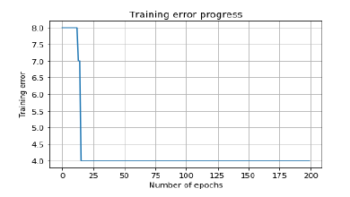
Train the neural network with number of epochs and learning rate as shown −

error = neural_net.train(data, labels, epochs = 200, show = 20, lr = 0.01)

Now, visualize and plot the training progress using the following commands −

plt.figure()
plt.plot(error)
plt.xlabel('Number of epochs')
plt.ylabel('Training error')
plt.title('Training error progress')
plt.grid()
plt.show()

Now, use the test data-points in above classifier −

print('\nTest Results:')
data_test = [[1.5, 3.2], [3.6, 1.7], [3.6, 5.7],[1.6, 3.9]] for item in data_test:
   print(item, '-->', neural_net.sim([item])[0])

You can find the test results as shown here −

[1.5, 3.2] --> [1. 0.]
[3.6, 1.7] --> [1. 0.]
[3.6, 5.7] --> [1. 1.]
[1.6, 3.9] --> [1. 0.]

You can see the following graphs as the output of the code discussed till now −

Multi-Layer Neural Networks

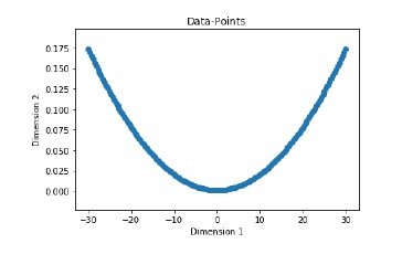
In this example, we are creating a multi-layer neural network that consists of more than one layer to extract the underlying patterns in the training data. This multilayer neural network will work like a regressor. We are going to generate some data points based on the equation: y = 2x²+8.

Import the necessary packages as shown −

import numpy as np
import matplotlib.pyplot as plt
import neurolab as nl

Generate some data point based on the above mentioned equation −

min_val = -30
max_val = 30
num_points = 160
x = np.linspace(min_val, max_val, num_points)
y = 2 * np.square(x) + 8
y /= np.linalg.norm(y)

Now, reshape this data set as follows −

data = x.reshape(num_points, 1)
labels = y.reshape(num_points, 1)

Visualize and plot the input data set using the following commands −

plt.figure()
plt.scatter(data, labels)
plt.xlabel('Dimension 1')
plt.ylabel('Dimension 2')
plt.title('Data-points')

Now, build the neural network having two hidden layers with neurolab with ten neurons in the first hidden layer, six in the second hidden layer and one in the output layer.

neural_net = nl.net.newff([[min_val, max_val]], [10, 6, 1])

Now use the gradient training algorithm −

neural_net.trainf = nl.train.train_gd

Now train the network with goal of learning on the data generated above −

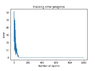
error = neural_net.train(data, labels, epochs = 1000, show = 100, goal = 0.01)

Now, run the neural networks on the training data-points −

output = neural_net.sim(data)
y_pred = output.reshape(num_points)

Now plot and visualization task −

plt.figure()
plt.plot(error)
plt.xlabel('Number of epochs')
plt.ylabel('Error')
plt.title('Training error progress')

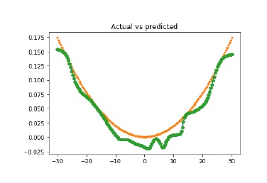
Now we will be plotting the actual versus predicted output −

x_dense = np.linspace(min_val, max_val, num_points * 2)
y_dense_pred = neural_net.sim(x_dense.reshape(x_dense.size,1)).reshape(x_dense.size)
plt.figure()
plt.plot(x_dense, y_dense_pred, '-', x, y, '.', x, y_pred, 'p')
plt.title('Actual vs predicted')
plt.show()

As a result of the above commands, you can observe the graphs as shown below −